Blog
21 Google Sheets Formulas For SEO To Speed Up Your Workflow
Simran Gill
11 December 2025
Google Sheets formulas are of the most powerful and versatile tools in any SEO’s toolset. Once Excel formulas were the the go-to, but Google Sheets offers much more versatility and some additional, very handy functions to have in your arsenal. Google Sheets is a great tool for many SEO applications and creating on-the-fly solutions to data extraction and manipulation of sizeable data sets.
In future posts we will venture into these more complex applications, but for this one, we’re just going to look at at the 21 best Google Sheets formulas for SEO that you can use in your day-to-day work to speed up your workflow.
1. VLOOKUP
This Google Sheets formula is a great time saver that you can use for consolidating large sets of data.
VLOOKUP stands for “Vertical Lookup” and can return relevant data from vertically presented data sets. (i.e. Column header, with data presented beneath).
An example of where this would be useful would be if you have a defined set of keywords that you are wanting to check, but you haven’t set up specific keyword tracking in SEMrush / AWR.
The VLOOKUP formula can return the relative data in reference to your search query.
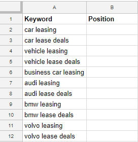
For example, you want to check these rankings for the hypothetical website “carleasingwebsite.co.uk”:
You have your nicely presented list of keywords:
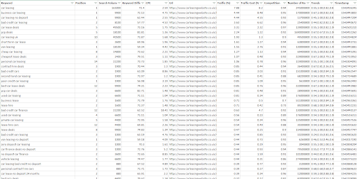
And you have this mass of keyword data from SEMrush:
You can nicely extract the relevant positions into your keyword list, using the following formula:
=VLOOKUP(searchkey,datarange,index,[is_sorted])
Searchkey: The item you want to look for.
Datarange: The area you want to look within – the first column in the range must be the one you want to search in.
Index: The column you want to return data from in your specified data range.
NOTE: If your range is A:D then 2 would = Column B.
If your range is C:F then 2 would = Column D.
Is sorted: FALSE – Returns only an exact match to the search key, otherwise returns ERROR.
TRUE – Assumes data is sorted and returns closest match for search key.
NOTE: As a general rule always use FALSE – you can use other formulas to handle the errors as you wish.
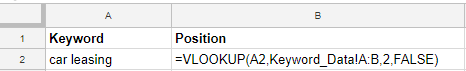
For this example the formula would look like this:
=VLOOKUP(A2,Keyword_Data!A:B,2,FALSE)
You can then copy the formula down (or use an ARRAYFORMULA) to show the results for your other keywords:
If you’ve specified a range with row numbers, make sure you lock the range with $’s before you starting dragging it around: =VLOOKUP(A2,Keyword_Data!$A$2:$B$12000,2,FALSE)
2. HLOOKUP
The HLOOKUP Google Sheets formula is much like the VLOOKUP formula. HLOOKUP stands for “Horizontal Lookup” and (you’ve probably guessed it) is used for extracting data from a horizontal range search.
This is useful for scanning columns of data, where you know the row you want to return but need to find the correct column.
For example, here we have the count of top ranking keywords for a lot of competitors:
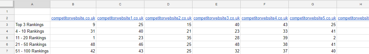
I want to find how many top 3 rankings competitorwebsite26.co.uk has, so we can use the following formula:
=HLOOKUP("competitorwebsite26.co.uk",B2:AC7,2,false)
This will search horizontally in row 2 for “competitorwebsite26.co.uk” and return the second row in that column – containing its top 3 rankings.
3. IF
The IF statement is the Google Sheets formula you will use most frequently. It’s the simple “If that – Then this” formula that you can use to query your data and instigate a reaction given a certain circumstance.
It would look like this:
=IF(logical_expression,value_if_true,value_if_false)
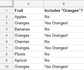
For example, here you have a list of fruit and you want to know which ones say “Oranges,” you could use this formula:
=IF(A2="Oranges","Yes Oranges!","No")
This is a very simple application, but fused with other functions can begin to create very useful results.
4. IFERROR
Sometimes your Google Sheets formulas will return an error – hey, it happens! – but fortunately the IFERROR function can help.
Wrapping your formulas in IFERROR allows you to perform another action, in the event that your formula returns an error, otherwise it will function as normal.
It works like this:
=IFERROR(“no error”,"error")
Just put your formula after the opening bracket and what you would like to happen should it throw an error after the comma.
A nice way of tidying up your data is to simply leave the “error” blank, so you can just see where your formula has run successfully.
5. IF ISNA VLOOKUP
Now you’ve got IF statements and VLOOKUP’s down, you can start stringing them together.
This is a useful one for checking if an item in one list exists in another list.
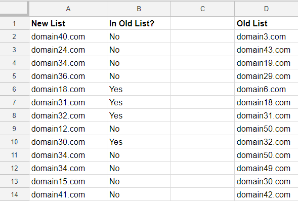
For example, if you’re updating a disavow file and want to check you aren’t re-including domains in your new list that have already been added to the file, use this:
=IF(ISNA(VLOOKUP(searchkey,range,index,FALSE)),"No","Yes")
The above formula checks if the search value is present in the old list and returns “Yes” or “No” depending on the outcome.
You can then just apply a filter and make sure you’re only adding new domains, keeping your disavow file nice and tidy!
6. RIGHT / LEFT
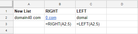
The RIGHT / LEFT Google Sheets function allows you to return a specified quantity of characters from either end of the cell contents.
It works like this:
=RIGHT(string,[number_of_characters])
For example:
Not very interesting yet, but wait…
7. LEN
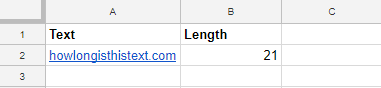
The LEN Google Sheets function returns the number of characters in a given cell. (Very useful for writing meta titles / descriptions and keeping in length).
It works like this:
=LEN(text)
For example:
=LEN(A2)
8. RIGHT + LEN
Combining RIGHT + LEN together has a very handy purpose. You’ve just downloaded your disavow file from Google Search Console and you want to check your new list against the old disavow file – but all of the domains have “domain:” strapped to the beginning.
Use this:
=RIGHT(A2,LEN(A2)-7)
Now you can scan, compare and check the domains as normal.
9. SPLIT
Use this Google Sheets formula to quickly split text using a specified delimiter.
It works like this:
=SPLIT(text,delimiter)
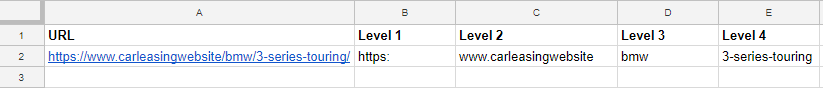
This allows you to quickly split URLs into their different levels.
For example, you have a list of URLs like this:
https://www.carleasingwebsite/bmw/3-series-touring/
And you want to split them so you have the car brands and models separately.
Use this:
=SPLIT(A2,"/")
10. SUBSTITUTE
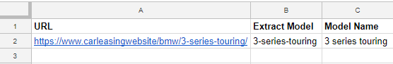
Maybe you’ve just extracted some words from a URL structure, as above, or perhaps someone’s just provided you with a strangely formatted keywords list; either way there’s a character you want to swap out.
Enter SUBSTITUTE.
It works like this:
=SUBSTITUTE(text_to_search,search_for,replace_with, [occurence number - optional])
If you’ve just extracted a portion of a URL, words will often be separated by hyphens.
Use this formula to remove them:
=SUBSTITUTE(B2,"-"," ")
11. CONCATENATE
The CONCATENATE Google sheets formula is simply the opposite of SPLIT – a joining function. Specify either several or a range of cells and it will join them together for you.
It works like this:
=CONCATENATE(string1,string2,string3)
Or
=CONCATENATE(range)
For example:
=CONCATENATE(A2:E2)
12. JOIN
You can use JOIN similarly to CONCATENATE, if you want to add a delimiter where you join the words.
It works like this:
=JOIN(delimiter,value_or_array)
For example:
=JOIN("/",A2:D2)
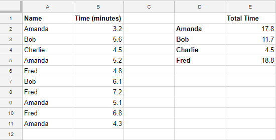
13. COUNTIF
COUNTIF allows you to count the number of instances of a value in a range.
Like this:
=COUNTIF(range,criterion)
For example:
=COUNTIF(A2:A8,C2)
This will count the number of times C2 (i.e. Amanda) appears in the range and can be dragged down to do the same for the other members in the list.
You can also use COUNTIFS to count using multiple criteria.
It would work like this:
=COUNTIFS(range_1,criteria_1,range_2,criteria_2,etc..)
For example, perhaps you want to count the number of times Amanda got a time of better than 5 minutes.
Your formula would look like this:
=COUNTIFS($A$2:$A$11,D2,$B$2:$B$11,"<5")
14. SUMIF
SUMIF works much like COUNTIF, however rather than counting the number of instances it will add them together.
It works like this:
=SUMIF(range,criterion,[sum_range])
For example, this formula will add together all of each runner’s times that were better than 5 minutes:
=SUMIF(A2:A11,D2,B2:B11)
As with COUNTIF, you can also use SUMIFS to add instances together on the basis of multiple criteria.
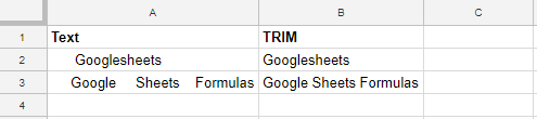
15. TRIM
Sometimes your formulas will throw errors when referencing cells. Perhaps your VLOOKUP can’t find an item you know is there, or perhaps COUNTIF isn’t counting all instances of an item.
After a long time searching, you discover it’s because you have erroneously added a space at the end of the cell contents.
Avoid this issue by using the TRIM function.
This works by removing leading, trailing and repeated spaces in text, like this:
=TRIM(text)
For example:
=TRIM(A2)
NOTE: It only removes repeated spaces within the text, leaving one with the assumption it is written text.
If you wish to remove all spaces, use SUBSTITUTE: =SUBSTITUTE(A3,” “,“”).
16. UPPER / LOWER / PROPER
While fixing issues and tidying up text, it seems wise to cover UPPER, LOWER and PROPER.
These Google Sheets formulas allow you to change the formatting of all text in a cell to either all upper case (UPPER), all lower case (LOWER), or capitalising the first letter of each word (PROPER), as in the examples below.
This can also help to reduce errors in case sensitive formulae.
17. UNIQUE
Another great function for speeding up your workflow is UNIQUE.
As the name would suggest this returns only unique values from a range.
Useful if you have a mass of keyword data from various competitors that you plan to query, but attempting to repeatedly query 300,000 rows of data repeatedly is really going to slow things down!
Use UNIQUE, like this:
=UNIQUE(range)
The great thing about unique is that it queries the entire row of specified data.
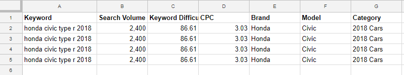
So, if you used the below formula on the following data set:
=UNIQUE(A1:G5)
These would all be unique values – as column G is different each time – and the output would remain the same.
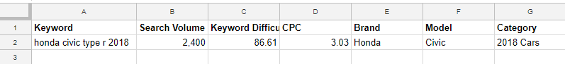
However, if you applied it to this data:
You would get the following, de-duplicated output:
18. ARRAYFORMULA
The ARRAYFORMULA Google Sheets formula is a great time saver! This allows you to apply most formulas that would otherwise only apply to a single cell to an entire range.
This reduces the likelihood of errors in your formulas and means you don’t have to delete and drag the formula across after every change you make!
And if you want to copy your formulas to a new sheet, you need only copy the top cells where your ARRAYFORMULAS exist. No need to try and drag your selector across to copy the whole sheet!
It works like this:
=ARRAYFORMULA(formula)
The only difference is you now specify a range in the enclosed formulae, as opposed to a singular cell.
An example of an ARRAYFORMULA with IF(ISNA(VLOOKUP)) would be:
=ARRAYFORMULA(IF(ISNA(VLOOKUP(A2:A,D2:D14,1,FALSE)),"Yes","No"))
Tip: Wrap your your formula inside the ARRAY in an IF(ISBLANK) statement, so it only shows a result where relevant.
Like this:
=ARRAYFORMULA(IF(ISBLANK(A2:A),"",IF(ISNA(VLOOKUP(A2:A,D2:D14,1,FALSE)),"No","Yes")))
19. IMPORTRANGE
Google Sheets, as brilliant as it is, can only handle so much – and that 5,000,000 cell limit will come around quicker than you’d think.
So, when you’ve either used all the available cells, and you’ve received this message:
or your sheet is just starting to lag:
you can use IMPORTRANGE to have your data continue in another workbook.
This means you can update your data in the first workbook and see it update in (almost) real-time in any of the sheets where you’ve used the IMPORTRANGE formula.
It works like this:
=IMPORTRANGE("spreadsheet_url","range_string")
For example:
=IMPORTRANGE("https://docs.google.com/spreadsheets/d/1eAZ6ofJgQNePyz6-KL-82UqNQWLVXRl7cqjrtvCJ8IU/edit","Sheet_Name!A1:H30")
After you’ve entered the formula, you’ll get a #REF! error. Simply hover over this and click “Allow Access” to join the sheets together.
And see your data appear:
NOTE: If there’s not enough room for the data to be imported or you try to write in the imported area, you will get an error, so make sure there’s enough room before you import.
If you only want to import certain columns of the data, you can combine IMPORTRANGE with the QUERY function for massive versatility.
20. QUERY + IMPORTRANGE
Using IMPORTRANGE and the QUERY function together can give you massive flexibility on how your data is imported.
You can choose which columns of data are imported, the order the columns appear, filter by numeric values, exclude rows with certain terms, and order by multiple columns.
QUERY allows you to use a Google Sheets version of SQL (Syntax Query Language) to query your data. QUERY can be used without IMPORTRANGE, but for this example we’re just looking at how you can speed up your use of this formula.
A standard QUERY + IMPORTRANGE formula would work like this:
=QUERY(IMPORTRANGE("sheet_url","range_string"),"QUERY")
For this example I have a large amount of keyword data around car leasing / hire / rental / finance / used cars terms. I have just downloaded it from SEMrush and it looks like this:
I only want to see the data for keywords with lease / leasing terms and a Search Volume of greater than 1000. I also want to remove any terms with “used,” and I am getting results for the brands “select car leasing,” “what car,” “hippo leasing” and “nationwide,” so I’d like to remove those as well. I’d also like to change the order of the results to only show: Keyword, Search Volume, CPC, Keyword Difficulty. Then I’d like to order the results by greatest Search Volume first.
It seems like a lot to ask and would take some time to go through each of the motions to achieve this manually.
So, if I wanted to achieve all of this simultaneously, I could use the following formula:
=QUERY(IMPORTRANGE("https://docs.google.com/spreadsheets/d/1jY2ZHLRS6l0YswGUfaBrmDN-c-Ums5V5FlUgAs0PM_o/edit","KeywordData!A1:H2000"),"SELECT Col1, Col2, Col4, Col3 WHERE Col1 contains 'leas' AND Col2 > 1000 AND NOT Col1 contains 'used' AND NOT Col1 contains 'select car' AND NOT Col1 contains 'what car' AND NOT Col1 contains 'hippo' AND NOT Col1 contains 'nationwide' order by Col2 desc")
NOTE: Make sure to type Col1 with a capital C, otherwise you’ll get an error.
The output is a much more relevant and manageable set of data:
The above formula used the following SQL functions:
SELECT: Specify the columns you would like to import – Use “SELECT *“ (without quotations) to import all columns.
CONTAINS: Cell contains specific text. – Use “=” instead of contains for exact match.
NOT: Use to specify an exclude parameter.
ORDER BY: Choose column to sort by – specify “asc” for ascending or “desc” for descending. You can sort using multiple columns: ie. “ORDER BY Col2 desc, Col1 asc”
The order you list the columns in will specify the hierarchy.
We will go into further depth with this formula in future posts, but it’s a simple formula you can use to speed up your work between sheets.
21. REGEXEXTRACT
REGEXEXTRACT is a very powerful function in Google Sheets. This allows you to use Regular Expressions to extract specific information from your data. The flexibility you can achieve using this is vast. However, getting to grips with Regular Expressions can take some time.
It works like this:
=REGEXEXTRACT(text,regular_expression)
A great way of beginning your categorisation for keyword research is by crawling a competitor’s site and extracting the top level categorisation data from their site to influence your initial research.
Find a competitor with a reasonable level of clarity in their URL structure and run a crawl – what we’re looking for is URLs that have a distinct key on either side of the portion that we’d like to extract.
Now you’ve run the crawl, you should have a list of URLs that will look something like this:
It’s a bit of a mess, but there is enough structure there to work with.
Preceding each of the destinations is this: “https://www.travel_website.com/destinations/”
Then we have the destination – which we would like to extract – which is followed by “/”.
We can then use these “hitpoints” in the following formula to extract our destinations:
=REGEXEXTRACT(A3,"https://www.travel_website.com/destinations/(.*?)/")
The small piece of Regex in the formula (.*?) allows us to match and return any character in between these two points.
We can then wrap this in SORT, SUBSTITUTE, PROPER, IFERROR, ARRAYFORMULA, and UNIQUE, to get a nice concise, ordered and properly capitalised list of destinations.
Like this:
=SORT(UNIQUE(ARRAYFORMULA(IFERROR(PROPER(SUBSTITUTE(REGEXEXTRACT(A2:A,"https://www.travel_website.com/destinations/(.*?)/"),"-"," ")),""))),1,TRUE)
Wrapping Up
I hope this guide has given you some useful tips that you can integrate into your day-to-day work to speed up your workflow in Google Sheets and I look forward to going into more depth for specific applications in future posts.
If you’d like any help with your SEO strategy, then please get in touch and we’ll be happy to help.
Written by
Simran Gill
Latest posts.


Contact.
We’re always keen to talk search marketing.
We’d love to chat with you about your next project and goals, or simply share some additional insight into the industry and how we could potentially work together to drive growth.